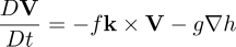
Here is Semi-Lagrangian method with bi-cubic interpolation, with filter for short wavelengths. In the semi-Lagrangian method, we follow new particles at every timestep. In pure Eulerian methods, we only focus on grid points. Bilinear interpolation leads to excessive smoothing, especially for shorter wavelengths. For SL methods, for uniform velocity, it is possible to take arbitrarily large timesteps, without violating CFL condition. Periodic grid with a mountain on the bottom of the ocean. The governing equations are
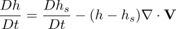
As seen these are the Lagrangian form of the equations, following trajectories of water particles. The semi-Lagrangian methods avoid some instabilities due to nonlinear terms, as they are eliminated in the Lagrangian expression. SL methods usually have a lot more computation at a single iteration step compared to a pure finite difference method. The main benefit of SL over FD is then when it allows a long enough timestep, so that the extra calculation time is compensated.
Simulation example
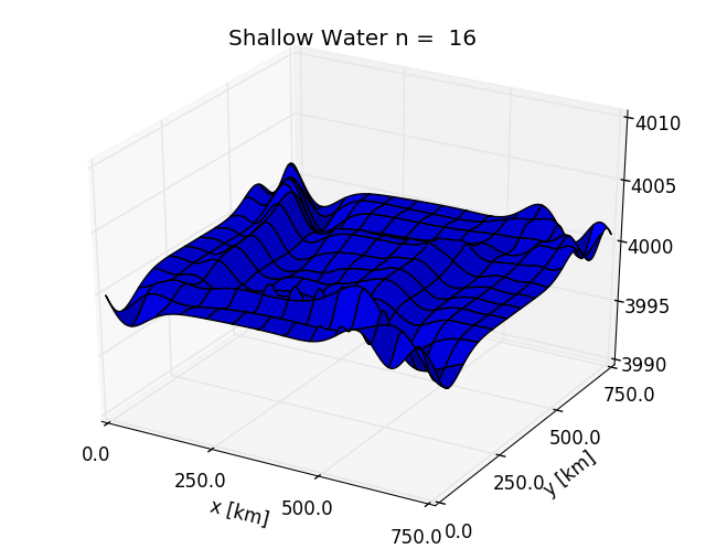
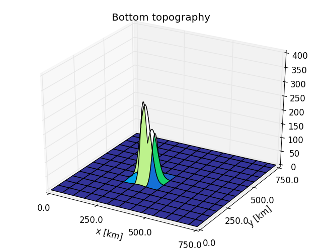
Mountain on the seabed
Bottom topography changes the the dynamics, and especially from a viewpoint of conservation of potential vorticity.
Oscillations due to Coriolis force
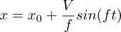
A particle under influence of coriolis force, and ignoring curvature effects and keeping a constant coriolis term, will undergo circular oscillations In the northern hemisphere, the motion will be clockwise(anticyclonal). The equations of motions are


The solution, for a particle starting at (x0,y0) with a horizontal speed V, will move according to
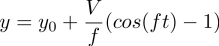
The SWE has more dynamics than just pure coriolis force, but the model captures the same oscillation in essence. The theoretical circular motion is plotted in green.