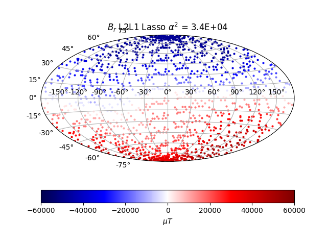
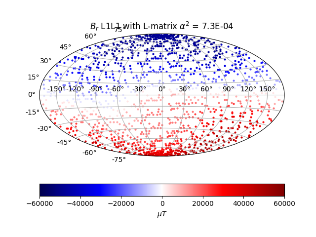
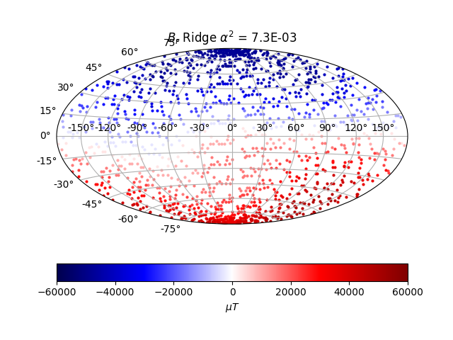
Magnetic field data captured by SWARM satellite. Downward continuation Robust estimation, iterated IRLS Overdetermined system. Conditioning numbers. The data consists of around 7500 observations, made in 2014, by a high-altitude satellite. The field data will be used to fit a model for the core surface boundary. This procedure includes downward continuation, which introduces instability and amplifies short wavelengths and observation noise. Thus regularization is required. We can start off with a simple inversion method, assuming gaussian noise and thus using L2-norm on the misfit, with L2-norm on the model. This is the classical Tikhonov (Ridge regression special case) method. Then we can try combinations of L1 norm and L2 norms on model and misfit. Around 97% of the magnetic field measured on Earth originates from internal sources. The core is too hot to sustain a permanent magnet, and instead much more difficult dynamics are at play, involving fluid dynamics along with the rotation of Earth. Note that this is a model for the radial field alone, where the magnetic field consists of also two angular directions. The radial magnetic field data can be seen below
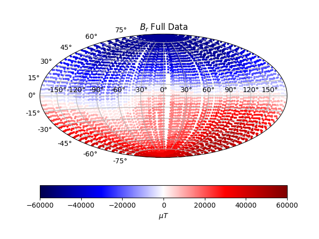
As can be seen from the data, putting aside errors, the radial magnetic field of Earth is largely a dipole, as from a north-south bar magnet. The north pole is the magnetic south pole, and vice verca. That situation changes with time however, as the field reverses on large timescales. The left figure is a solution with almost no regularization, and the right figure is a solution with too much. The predicted field is squished towards zero, leaving the amplitudes smaller, and also create a strong bias beyond any physically reasonable solution.
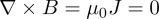
From Maxwell's equations, the curl of the magnetic field is zero in a region free from current sources, or constant electric field, The model can be derived from some simple physical considerations and assumptions.
Magnetic measurements on the satellite are done with shielding from electronic, to shield the measurement device as much as possible from the electromagnetic noise from the satellite itself. For zero curl, the field can be written as gradient of a potential field,

The magnetic field is divergence free,

And so we can arrive at Laplace's equations


The parameters of the model are the g's and h's. For a SH model of degree n = 20, without intercept, there will be 440 model parameters. About 20 degree SH model is reasonable for a model at the surface of Earth. Only internal sources are modelled, i.e magnetic disturbances from the ionosphere, the influence of the sun etc. is not modelled, but will be present as variance in the data. With up to 7561 data points we thus have an overdetermined system. For computational efficiency, only around 750 points will be used, at the cost of more uncertainty in the results. The sum of spherical harmonics, with radius coefficients, will make up the design matrix G, that is used in the inverse steps to find the model m, which consits of the g's and h's. The radius factor is seen with reference from the surface of earth, with a = 6371km, and while the data is collected at around 6800km by the sattelite, and also consideration of the field at the core-mantle boundary will be given, which is at a radius of 3480km. Thus the inverse problem uses both downward continuation and upward continuation. Downward continuation to the CMB is an unstable process, which gives weight to higher frequencies, as will be seen in some of the methods.
Best solution - IRLS L1L1 norm with L matrix
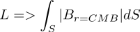
The best solution comes from using the L1 norm on misfit and L1 norm on the total magnetic flux at the core-mantle boundary The solution will be given by the IRLS algerithm, updating the W and Wm matrix at each step, using e.g Huber weights. The W matrix is a data weight matrix, which makes the solution robust to outliers.

The L-matrix is given by the discretisation of the integrated unsigned magnetic flux. The radial field at the CMB is actually just the predicted values Bcmb = Lm, so the L matrix is similar to the design matrix G, but at a different radius, longitude and latitude.
It's also possible to do regularisation on the integrated squared radial field. The solution for reasonable regularisation parameter is seen below
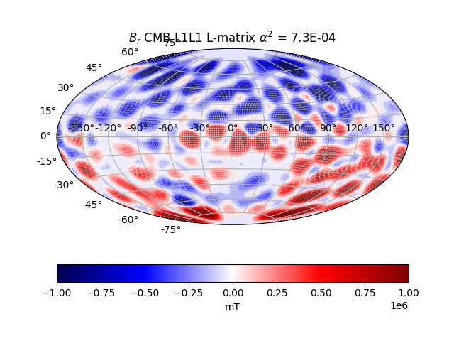
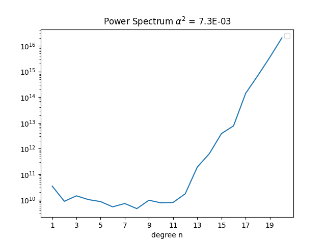
We can see that it captures the Earth surface field as we know it pretty well. The radial field is also largely dipolar at the CMB, with some large persistent reverse magnetic flux areas on the southern hemisphere, which is consistent with theory and the field at the surface. The geomagnetic power spectrum at the core-boundary surface for the chosen solution is
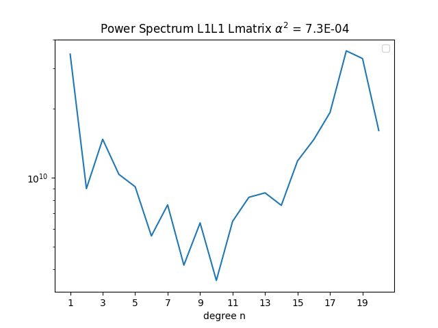
It's best to downward continue the Earth Surface field at to the core-mantle boundary, if there is no field generated in the mantle and the curst. (Lowes,1974) I.e no sources of Br in between. There are small but significant sources to the surface field, from magnetized crustal rocks. We can expect the crustal field to exist mostly of higher harmonics, due to its shallow origin. Early estimates showed the crustal field to mostly show itself from n = 25 and upwards, to e.g n = 500. We mostly expect the core field to be flat or slowly decreasing up to n = 10, at the core field, corresponding to nearly a 'white' spectrum from the sources at radius 0.47a, with maybe a slight increase for n = 2, due to a deeper dipole source at 0.35a The earth surface spectrum decreases up to between n = 14 to 20, with main contributions from the core field. The ES spectrum then stays nearly flat from n = 20. And the core field is greater than the crustal field to at least n = 11, while the crustal field likely has very low contribution for small n. According to (Langel & Estes 1982) we see to distinct slopes at Earth Surface magnetic field spectrum, with a distinct change at n = 14. The spectrum before that comes mostly from core field sources, and the spectrum after n = 15 from crustal sources. It is difficult to observe the core field after n = 14, because the crustal field obscures it. External sources include ionosphere and magnetosphere. The Earth Surface spectrum, the dipole term stands way higher than the rest, and a break near n = 14. The higher degrees are not due to noise in data, but carry actual meaningful physical information. The crustal field thus puts a limitation on our ability to estimate the core field, mostly for higher frequencies. The core spectrum should decrease slightly up to n = 14, and after that, increase fast. For n = 13 and 14, the crustal field still contributes a lot to the core spectrum.
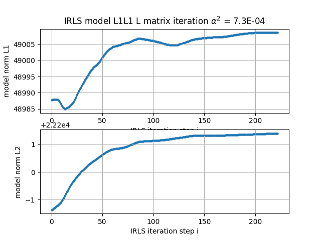
The IRLS algorithm updates two weight matrices, W for misfit and Wm for generalized model norm. The convergence criteria is a relative change in model norms, within E-7. After 200 steps the algorithm seems to have converged.
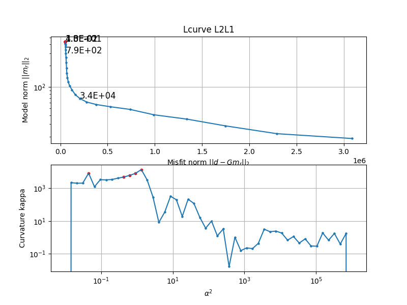
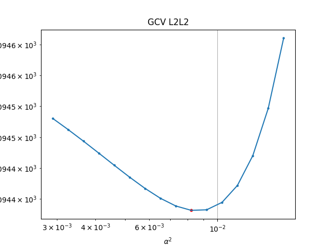
To great relief the Lcurve and GCV actually give pretty similar results, they both suggest a parameter close to E-4.
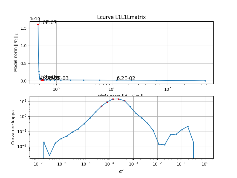
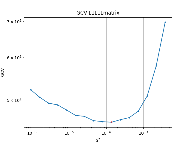
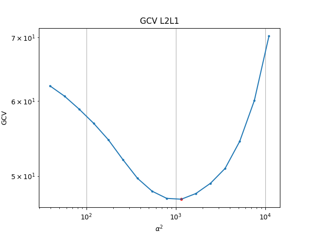
Regularization is basically a tradeoff between variance and bias. A least squares solution is often an overfit to the data. The obtained model has high variance and thus is very sensitive to small changes in data. Some authors plot log scales, some use no log scales, and some authors pick the value visually. The L-curve basically measures the misfit against the modelnorm. It's one way of choosing which regularization parameter to choose. The optimal regularization parameter, in this context, would be the one that balances the two norms, and would found on the corner of the curve. Getting a good sharp curve can be difficult, so some authors they pick a regularization parameter visually that most seems to represent the point where a balanced tradeoff happens. Another way of choosing parameter is the GCV, which is a generalization and more efficient way of doing Leave-One-Out cross validation. Basically measuring how well the model can predict a data point, if you had deliberately taken it out of the training set. The optimal parameter minimizes the GCV, which means on average, with splitting up the training set, you would have the lower residual sum of squares for that particular regularisation parameter. The GCV uses a denominator which essentially counts the effective degree of freedom, which the regularisation parameter also affects.
L2L2 norm Ridge Regression
One of the earliest methods to in regularized regression, in reducing variance, is the Ridge regression. To reduce variance of predictions and model parameters, we can put a penalty on the sum of squared parameters, next to the penantly on misfit. It can be expressed in the lagrangian form as

The advantage to the Ridge regression is the simple analytical solution, which can be cleanly expressed, without having to use iterative methods

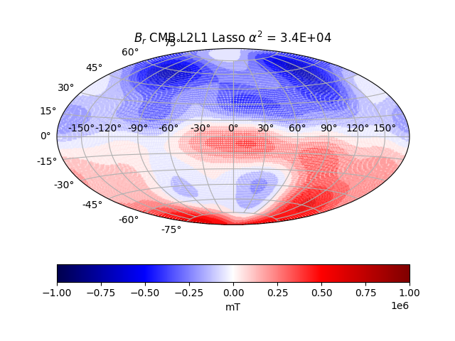
The predicted space data and CMB data for a particular regularisation parameter is chosen below.
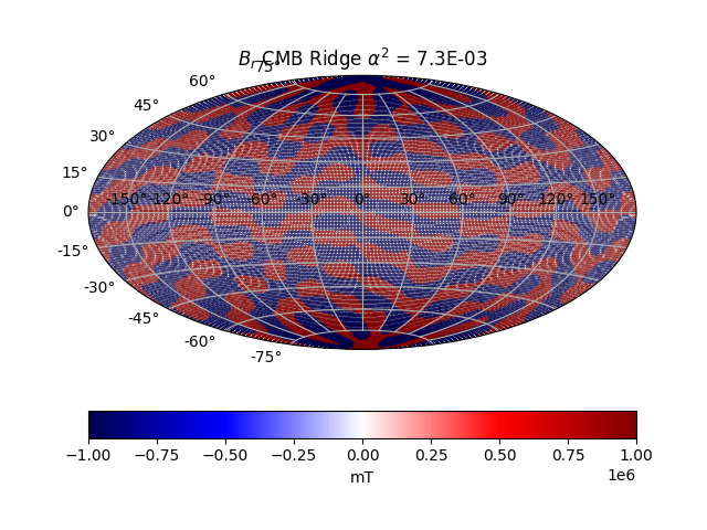
The solution at satellite height matches the data well visually, at least. At CMB level, the solution makes no sense, with higher frequencies dominating. It looks physically unreasonable, knowing what the surface and satellite height field looks like. The CMB field should still largely be dominated by a dipolar mode.
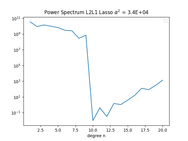
The power spectrum for the first 10 degrees is not too bad, despite the very unphysical fit at CMB level. The rise for larger spherical harmonics is due to crustal field sources.
The Ridge regression is fast to compute, since we do not need to iterate and converge. We can try for many parameters, and over a very long range. For a large range, spanning 10^-5 to 10^5, a corner is seen somewhere around 10^3.
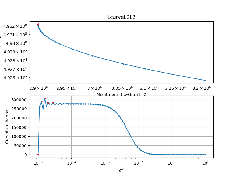
The L-curve is one method for parameter selection in regularized optimization problems. In its simplest form it shows the tradeoff between misfit and model norm, as the regularization parameter changes. As the regularization parameter increases, the model parameters decrease in size, and eventually m->0, and then Gm = Y -> 0, the predicted values will also approach zero. The misfit norm will approach ||d||_2, as the predicted values will be approach 0. Note that the different regularization methods use different terms on the axis, with appropiate weight matrices W,Wm included in the norms.
L2L1 norm Lasso regression
Putting L1 norm on model parameters gives the Lasso method. The Lasso method will do shrinkage as the Ridge regression, but also more directly feature selection, as it puts parameters to zero. The Lagrangian form can be expressed as

The solution for some parameter that is somewhat close to the optimal one given by Lcurve and GCV is seen below.