Markowitz Portfolio Theory is an application of constrained optimization to asset investment. We assume that with each asset there is an expected return, but also a variance in return(and perhaps negative return), which we call the risk of the asset. The Android app is made here using Python with Kivy. Buildozer is required to convert the project to an .apk file for the smartphone. Buildozer only works in Linux, so the project is made in Ubuntu runing on VirtualBox. It could probably be done in WSL too. Normally, SciPy handles constrained optimization very well, especially for this type of small example/school problem. Due to SciPy calling Fortran and other things, it is kinda difficult to combine with Kivy and Android. So we have to make our own optimizer algorithm using just NumPy, to solve inequality constrained QP. Our selfmade QP solver solves QP with inequality constraints as an iterated equality-constrained QP, and here we're using Primal Active-Set method. Numpy doesn't have LU decomposition, so we just invert the KKT matrix. It is hopefully stable enough for our small problem. x = [x1,x2,x3,x4,x5]^T is the fraction of available funds that are invested correspondingly to asset 1,2,..5. A strategy where we don't go short, and only hold long positions, correspond to inequality constraints xi>=0 for i each asset. Variants of MPT is still used today in some investment banks. Since returns are usually greater on a greater timescale, if one plans to hold positions for e.g a year, it is probably best to calculate statistics on a yearly basis. I.e don't use daily returns to calculate variance and expectation values, if the strategy is to hold for a year or more.
The method running on an Android smartphone is shown below. Making a great plot is difficult without Matplotlib, so now the data is just drawn on canvas. The upper part of the curve is the Efficient Frontier. For an expected return, one can see the associated risk. On the other hand, for an acceptable risk, one can see the greatest expected return.
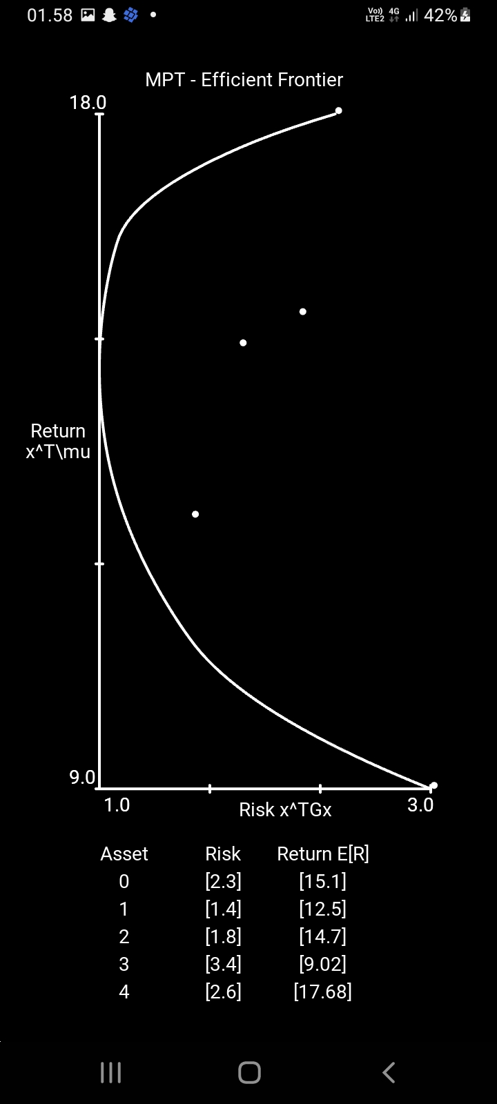
The best line found can be seen separating the two clusters of data. The line doesn't look like it's the optimal solution. To find the solution we inverse the KKT system, which probably causes instability and bad convergence. The problem can be formulated as Quadratic Programming with linear equality and linear inequality constraints. The efficient frontier is calculated by optimizing the portfolio, i.e solving the constrained optimization problem, for a range of chosen expected portfolio returns R.
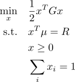
mu vector is the expected return of each asset, which with the fraction vector x, gives the total return R of the portfolio.
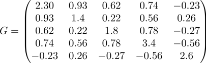
The matrix G is the variance-covariance matrix of each asset. Some assets have a higher risk, corresponding to a higher variance. And some assets can move with long-term strong correlation, if they e.g in the same or inter-dependent industries.
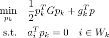
Active-Set method for inequality-constrained QP
A general QP problem(Nocedal & Wright ch. 16) can be written as
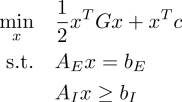
We can solve this as an iterated equality-constrained QP problem, which has known solutions. At each iteration, different constraints may be active, and this method is called the Primal Active-Set method. Since at each step a different number of constraints may be active, the size of the KKT matrix can change on each iteration.
The matrices are the equality constraint matrix and the inequality-constraint matrix, which is just the identity matrix that makes sure that each investment is positive, corresponding to going long on the asset.
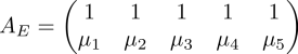
The matrices AE and AI contain our equality and inequality constraints. At any given iteration, only a subset of these constraints will be active. We will put them in a working set Wk. We can then make a new matrix composed of active constraints of both AE and AI. And the variables h and g are

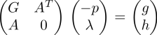
The KKT is written below, and corresponds to the first derivative and second derivatives of the cost function and the constraints. The system is here solved by direct inversion, which is far from ideal, but does use only numpy.
Before taking another step, we calculate the longest step we can take without violating any inequality constraints that are not currently in the working set.
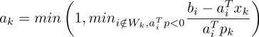
The step is then
On each step the active working set will be updated. Since parts of the algorithm compare numerical value to zero, a small threshold value is selected.