This section describes Support Vector Machines and a simple implementation in Python with Kivy, to use in Android Apps. SVM optimizes the decision boundary in the sense that it maximizes the distance from the line to both sides of the datapoints. Many other decision lines do not achieve this aspect. The linear SVM can only handle linearly separable datasets. To handle more difficult data, SVM with kernels are commonly used. Linear SVM is here implemented using just NumPy. Scipy and scikit-learn require multiple dependencies to work on Android, where as getting numpy to work is more straight forward. The solver and implementation is described in more detail at www.happimix/AndroidMPT/MPT.html. Here we solve the SVM using the primal formulation without slack variables. The primal formulation of the optimization problem is not often used, mostly because the dual formulation cna handle incorporation of different kernels.
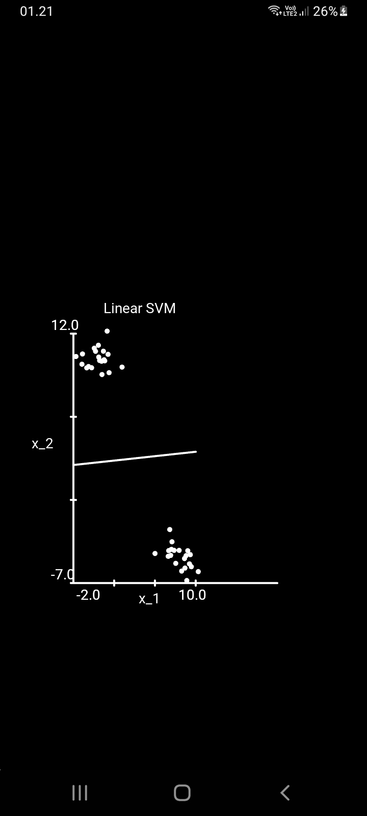
The method running on an Android smartphone is shown below. Making a great plot is difficult without Matplotlib, so now the data is just drawn on canvas.
Let points for class 1 with y = 1 satisfy w^Tx+b=1 and those with y = -1 satisfy w^tx+b=-1. The equations describe two parallel hyperplanes, that each separate the two classes of datapoints. The distance
is the distance from a point x to the plane described by w. In linear SVM, the look at the two planes that that parallel to eachother, where one plane touches one or more points in a given class. The distance between the two planes is then D = 2/||w||. The goal is to find the parameters w that maximize this distance. Maximizing 1/||w|| is rewritten as minimization of w^Tw. The problem is then formulated as Quadratic Programming with linear equality and linear inequality constraints.
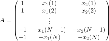
We use +w0 instead of +b or -b as is more commonly used, since to use the Primal Active Set method, we need to incorporate the constant into the constraint matrix and thus add a column of +1 or -1 to the feature x observations. The maximization problem above is rewritten as minimization QP problem, and the inequality constraints can be collected in a single expression
The intercept is now included into the feature vectors by adding 1 and -1 in the first column. Setting the points of class y = 1 as the first half of the matrix and the data for y = -1 as the lower half of the matrix, we have
This puts our problem into a useable form for our Active-Set QP iterative solver. We can use an initial feasible guess for parameters w, and then iterate equality-constrained QP problems to solve the inequality-constrained QP problem below

Note that our method has no equality constraints. The method is started with a horizontal line, until the optimal is found. The parameters are noted at the bottom of the app.